As I mentioned earlier, molecular dynamics simulation basically solves the Newtonian equation of motion. According to Newtonian physics, we can calculate force from the derivative of potential energy ( ![]() ). The energy of an atomistic system is the function of its electronic structure and is called electronic energy. Thus, we need to determine electronic energy first. In classical molecular dynamics simulation, electronic energy is considered a parametric function of the nuclear coordinates rather than the result of solving the laborious Schrodinger equation. The MD parameters can be fit to match experimental or high-level ab initio pre-computed data.
). The energy of an atomistic system is the function of its electronic structure and is called electronic energy. Thus, we need to determine electronic energy first. In classical molecular dynamics simulation, electronic energy is considered a parametric function of the nuclear coordinates rather than the result of solving the laborious Schrodinger equation. The MD parameters can be fit to match experimental or high-level ab initio pre-computed data.
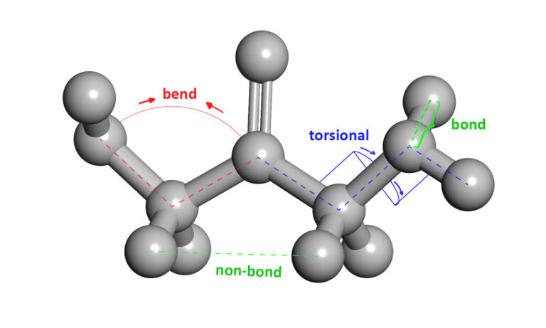
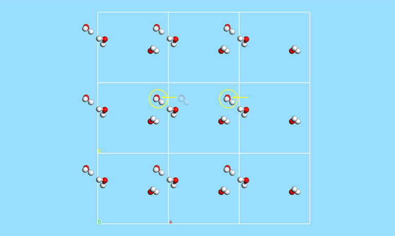
A force field is a combination of certain parametric functions and their parameters, defining the interaction between the system’s particles. The force field functions consist of bonded, non-bonded, and cross terms, each describing the energy required to distort the molecular system in a specific way (figure 3).
The bonded terms are the stretch, bending, and torsional terms, and non-bonded terms are the van der Waals and electrostatic terms. Finally, the cross-terms describe the coupling between the bonded terms. Different force fields utilize similar functional forms for each term; for example, many force fields use Morse potential as the stretch function or Lennard-Jones potential as the van der Waals function, but each has a unique set of parameters.
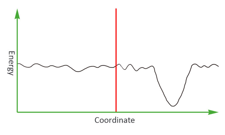
Having forces acting on each particle, you can solve Newton’s equation of motion. However, solving the equations for numerous particles simultaneously is not as easy as the problems of classical physics textbooks; therefore, we need an efficient way to deal with the equations. An Integration scheme is basically an approximate approach to solve Newton’s equations of motion for a poly-particle system. Various Integration techniques have been devised. One of the best yet simplest strategies, the Verlet algorithm is simply the Taylor expansion of particles’ coordinates around time 25.
![]()
The Verlet algorithm is a very efficient way of solving the equation of motion; however, its estimation of the new position contains an error of the order of t2. A more complicated algorithm, the velocity-Verlet algorithm, incorporates particles’ velocity into the scheme to reduce the error to the order of
![]()
A few more accurate integration schemes have been invented, Still, all of them are approximate methods, and you should bear in mind that the estimation error always increases rapidly with the time step.
References
- J. W. Ponder, D. A. Case, "Force Fields for Protein Simulations", Advances in Protein Chemistry, 66, 27-85.
- A. D. MacKerell et al., "All-Atom Empirical Potential for Molecular Modeling and Dynamics Studies of Proteins", The Journal of Physical Chemistry B, 102, 3586-3616.
- L. D. Schuler, X. Daura, W. F. van Gunsteren, "An improved GROMOS96 force field for aliphatic hydrocarbons in the condensed phase", J. Comput. Chem., 22, 1205-1218.
- W. L. Jorgensen, D. S. Maxwell, J. Tirado-Rives, "Development and Testing of the OPLS All-Atom Force Field on Conformational Energetics and Properties of Organic Liquids". J. Am. Chem. Soc. 118, 11225–11236.
- S. Riniker, "Fixed-Charge Atomistic Force Fields for Molecular Dynamics Simulations in the Condensed Phase: An Overview", Journal of Chemical Information and Modeling, 58 , 565-578.
- T. A. Halgren, W. Damm, "Polarizable force fields", Current Opinion in Structural Biology, 11, 236-242.
- N. Gresh et al., "Anisotropic, Polarizable Molecular Mechanics Studies of Inter- and Intramolecular Interactions and Ligand-Macromolecule Complexes. A Bottom-Up Strategy", Journal of Chemical Theory and Computation, 3, 1960–1986.
- "Anthony Stone: Computer programs". www-stone.ch.cam.ac.uk
- J. R. Maple et al., "A Polarizable Force Field and Continuum Solvation Methodology for Modeling of Protein-Ligand Interactions", Journal of Chemical Theory and Computation, 1, 694–715.
- J. Gao, D. Habibollazadeh, L. Shao, "A polarizable intermolecular potential function for simulation of liquid alcohols". The Journal of Physical Chemistry, 99, 16460–7.
- L. Yang et al., "New-generation amber united-atom force field", The Journal of Physical Chemistry B, 110, 13166–76.
- S. Patel, C. L. Brooks, "CHARMM fluctuating charge force field for proteins: I parameterization and application to bulk organic liquid simulations", Journal of Computational Chemistry, 25, 1–15.
- J. Barnoud, L. Monticelli, (2015) "Coarse-Grained Force Fields for Molecular Simulations. In: Kukol A. (eds) Molecular Modeling of Proteins. Methods in Molecular Biology (Methods and Protocols)", vol 1215. Humana Press, New York, NY.
- J. Barnoud, L. Monticelli, (2015) "Coarse-Grained Force Fields for Molecular Simulations. In: Kukol A. (eds) Molecular Modeling of Proteins. Methods in Molecular Biology (Methods and Protocols)", vol 1215. Humana Press, New York, NY.
- S. J. Marrink et al., "The MARTINI force field: coarse grained model for biomolecular simulations". The Journal of Physical Chemistry B., 111, 7812–24.
- D. Leonardo et al.,"SIRAH: A Structurally Unbiased Coarse-Grained Force Field for Proteins with Aqueous Solvation and Long-Range Electrostatics", Journal of Chemical Theory and Computation, 11, 723-739.
- A. Korkut, W. A. Hendrickson, "A force field for virtual atom molecular mechanics of proteins", Proceedings of the National Academy of Sciences of the United States of America, 106, 15667–72.
- Español, P. Warren, "Statistical Mechanics of Dissipative Particle Dynamics", Europhysics Letters, 30, 191–196.
- Senftle et al. "The ReaxFF reactive force-field: development, applications and future directions". npj Comput Mater 2, 15011.
- Warshel, R. M. Weiss, "An empirical valence bond approach for comparing reactions in solutions and in enzymes", Journal of the American Chemical Society, 102, 6218-6226.
- C. T. van Duin, S. Dasgupta, F. Lorant, W. A. Goddard, "ReaxFF: A Reactive Force Field for Hydrocarbons", The Journal of Physical Chemistry A, 105, 9396-9409.
- Behler, M, Parrinello, "Generalized Neural-Network Representation of High-Dimensional Potential-Energy Surfaces", Phys. Rev. Lett. 98, 146401.
- V. Botu et al., "Machine Learning Force Fields: Construction, Validation, and Outlook, The Journal of Physical Chemistry C", 121, 511-522.
- J. Behler et al., "Perspective: Machine learning potentials for atomistic simulations", J. Chem. Phys., 145, 170901.
- D. Rapaport, "The Art of Molecular Dynamics Simulation" (2nd ed.), Cambridge: Cambridge University Press.
- H. C. Andersen, "Molecular dynamics simulations at constant pressure and/or temperature", J. Chem. Phys. 72, 2384.
- W. G. Hoover, "Canonical dynamics: Equilibrium phase-space distributions", Phys. Rev. A, 31, 1695.
- H. J. C. Berendsen et al., "Molecular dynamics with coupling to an external bath", J. Chem. Phys. 81, 3684-90.
- G. Bussia, D. Donadio, M. Parrinello, "Canonical sampling through velocity rescaling", J. Chem. Phys. 126, 014101.
- H. J. C. Berendsen et al., "Molecular dynamics with coupling to an external bath", J. Chem. Phys. 81, 3684-90.
- M. Parrinello, A. Rahman, "Polymorphic transitions in single crystals: A new molecular dynamics method, Journal of Applied Physics", 52, 7182.
- J. Chen, 2018 IOP Conf. Ser.: Earth Environ. Sci., 128, 012110.
- John von Neumann Inst. for Computing, NIC series 1., IV, 562 S. (2000).
Hi
Hello. And Bye.
Congratulations. Great content.
An attractive alternative is to work with an atomic-level computer simulation of the relevant biomolecules. Molecular dynamics MD simulations predict how every atom in a protein or other molecular system will move over time, based on a general model of the physics governing interatomic interactions Karplus and Mc Cammon, 2002. These simulations can capture a wide variety of important biomolecular processes, including conformational change, ligand binding, and protein folding, revealing the positions of all the atoms at femtosecond temporal resolution.
In general, a small thermostat timescale parameter causes a tighter coupling to the virtual heat bath and a system temperature that closely follows the reservoir temperature. Such a tight thermostat coupling is typically accompanied by a more pronounced interference with the natural dynamics of the particles, however. Therefore, when aiming at a precise measurement of dynamical properties, such as diffusion or vibrations, you should use a larger value of the thermal coupling constant or consider running the simulation in the NVE ensemble to avoid artifacts of the thermostat.
Bravo!!
I just want to say thank you for this great website. I found a solution here on insilicosci.com for my issue.